Quick start

Quick start#

Installation#

The Python module can be directly installed from PyPI with:

pip install anta_database

Note that this module was developed for Python versions >=3.11. It is also recommanded to install it in a dedicated fresh python environment to avoid dependency issues.

This Python module is designed to query, filter, and visualize data stored in an AntADatabase folder. While the AntADatabase is not yet publicly available, you can contact me for access to test the tool. You can already have a look at this guide to have an idea of the features of this tool. This Jupyter Notebook can be directly downloaded (top bar) and ran locally (assuming you had downloaded or compiled the AntADatabase folder).

Initializing the database#

Having the AntADatabase folder stored on your machine, you can initialize import and initialize the ‘Database’ class which provides SQL query and filter functions as well as quick visualization function.

# Initialize the database and create the SQL table (required only once or when adding new datasets)
from anta_database import Database

db = Database('/home/anthe/documents/data/isochrones/AntADatabase/', index_database=True)

 Found 11903 files to index

Note: the index_database=True argument creates a SQLite table (AntADatabase.db) that indexes all datasets in the AntADatabase folder. This ensures that future queries reflect data that is actually present in AntADatabase. This allows you to download the current entire AntADatabase or parts of it. You only need to set index_database=True once or when you add new datasets to the folder.

# For subsequent uses (no need to re-index unless new datasets are added)
db = Database('/home/anthe/documents/data/isochrones/AntADatabase/')

Querying the database#

This section provides examples for querying the database using the query() and filter_out() functions. These functions allow you to browse and filter data based on various criteria such as datasets, institutes, projects, regions, layer ages and more.

Use the query() without argument for an overview of the entire data:

db.query()

Metadata from query:

  - dataset: Ashmore_2020, Beem_2021, Bodart_2021, Bodart_2025a, Bodart_2025b, Cavitte_2020, Chung_2023, Franke_2025, Jacobel_2005, Leysinger_Vieli_2011, Muldoon_2023, Mulvaney_2023, Sanderson_2024, Siegert_2004, Wang_2023, Winter_2018, Yan_2025

  - institute: AWI, BAS, LDEO, NASA-CRESIS, PRIC, PRIC-UTIG-AAD, SPRI-NSF-DTU, St-Olaf-College, UA, UTIG, UTIG-AAD

  - project: AGAP-NORTH, AGAP-SOUTH-GAMBIT, AGASEA, ANTR, ATRS, BBAS, BE-OI, CHARISO, GIMBLE, ICECAP, ICECAP-OIA, ICECAP2, IMAFI, OIB, POLARGAP, PPT, SNACC-DML, SOAR-CASERTZ, SOAR-DVD, SPC, US-ITASE, WISE_ISODYN, nan

  - acquisition_year: 1970-1979, 1974-1978, 1998-2008, 1999-2025, 2001-2002, 2004, 2005, 2005-2019, 2007-2016, 2009, 2010, 2011, 2012, 2013, 2016, 2016-2018, 2016-2019, 2017, 2018, None

  - age: 800, 2615, 3100, 4700, 4720, 4800, 5600, 6400, 6500, 6940, 7200, 7400, 8500, 9500, 10000, 10001, 10516, 10700, 11100, 12000, 13200, 13500, 15000, 15400, 16000, 16500, 16800, 17500, 17532, 18000, 23500, 25600, 29100, 29400, 30397, 31400, 36300, 36500, 37600, 38000, 38100, 38200, 38500, 39215, 43600, 46400, 47110, 48300, 51400, 52200, 62235, 62477, 64400, 72500, 73000, 73300, 73400, 73500, 74200, 75160, 75300, 80007, 82000, 82646, 84300, 90000, 90200, 90400, 91000, 93900, 95500, 96500, 97667, 106300, 108315, 113000, 117400, 118342, 121000, 121100, 127800, 128400, 128542, 129000, 132000, 135600, 160000, 160400, 161100, 161900, 166112, 166400, 169100, 170514, 179000, 200100, 202334, 203000, 215000, 220100, 239000, 240397, 243000, 244718, 254500, 262159, 277900, 304000, 320000, 326168, 327300, 336000, 341500, 345462, 352358, 365000, 366500, 381523, 395802, 396000, 399500, 414644, 419800, 473000, 482700, 516800, 560200, 611000, 708500

  - age_unc: -, 305, -, -, 280, 620, -, -, 600, 310, 100, 800, 900, 800, 300, 800, -, -, 100, 800, 400, 900, 1000, 1190, -, 790, -, -, -, 900, 1700, 100, -, 900, -, 3000, 3600, -, -, 800, 100, 600, 2200, -, 4900, 900, -, 1200, -, 100, -, -, 3000, -, -, -, 880, 2200, 1700, -, 7000, -, 1600, -, -, -, 1600, 3570, 1100, -, 7500, -, -, 1900, -, -, 1200, -, -, 1800, 1800, 3600, -, -, -, 10300, -, 3900, 3500, 6760, -, 3600, 19000, -, -, 2600, -, -, -, 3300, -, -, -, -, 5500, -, 4900, -, -, -, 4100, -, 5600, -, -, -, 7900, -, -, -, 9700, -, 13700, -, 22100, 21900, 27200, 35400, 54000

  - var: BASAL_UNIT, BED_ELEV, ICE_THK, IRH_DEPTH, IRH_NUM, SURF_ELEV

  - region: EAIS, WAIS

  - IMBIE_basin: A-Ap, Ap-B, B-C, C-Cp, Cp-D, D-Dp, Dp-E, E-Ep, Ep-F, G-H, J-Jpp, Jpp-K, K-A

  - radar_instrument: AWI-UWB, DELORES, EMR, HICARS, LDC-VHF, MCORDS, PASIN, SPRI-NSF-DTU-radar, nan

  - flight_id: 19993104, 20022106, BH05E-BH05B_proc2, W18, V18B-V18E, B14, 19972206, BH43B-BH43E_proc2, IRH_20172046, THW_SJB2_Y47b, OIA_JKB2n_Y64a, W08, THW_SJB2_X59a, B7, EPICA_IV_24, c09b, HRA3-HRA5_proc2, 20181022_01_001_025, W25, THW_SJB2_X81a, 20161109_03_026_049, HRB2-HRB7-2_proc2, PNV11___, BH47E-BH47B_proc, W16, [ ... ] , W23, 20181227_03_001, THW_SJB2_Y37b, OIA_JKB2n_Y74a, 19972406, B9, SOUTH_PATCH_FLOW_LINE_proc2, VCD_JKB2g_X08b, ROUTE4_proc2, IRH_20172047, 19993109, c11f, H42B-2H42E_proc2, 20173002, c20b, W26, 19983205, c20a, RAID2-BH01E_proc2, c12a, c10h, 2H30E-H30B, LSE_GCX0f_Y63a_depth, LSE_JKB2u_X59a_depth, 20231211_01_017 (found 832, displayed 50)

  - reference: Ashmore et al. (2020), Beem et al. (2021), Bodart et al. (2021), Bodart and Sutter (2025a), Bodart and Sutter (2025b), Cavitte et al. (2020), Chung et al. (2023), Franke et al. (2025), Jacobel and Welch (2005), Leysinger-Vieli et al. (2011), Muldoon et al. (2023), Mulvaney et al. (2023), Sanderson et al. (2024), Siegert and Payne (2024), Wang et al. (2023), Winter et al. (2018), Yan et al. (2025)
  - dataset DOI: https://doi.org/10.5281/zenodo.4945301, https://doi.org/10.15784/601437, https://doi.org/10.5285/F2DE31AF-9F83-44F8-9584-F0190A2CC3EB, https://doi.org/10.5281/zenodo.17348976, https://doi.org/10.5281/zenodo.17348094, https://doi.org/10.15784/601411, https://doi.pangaea.de/10.1594/PANGAEA.957176, https://doi.org/10.1594/PANGAEA.973266, https://doi.org/10.7265/N5R20Z9T, https://doi.org/10.5281/zenodo.15516203, https://doi.org/10.15784/601673, https://doi.pangaea.de/10.1594/PANGAEA.963470, https://doi.org/10.5285/cfafb639-991a-422f-9caa-7793c195d316, https://onlinelibrary.wiley.com/doi/10.1002/esp.1238, https://doi.org/10.1594/PANGAEA.958462, https://doi.org/10.1594/PANGAEA.895528, https://doi.org/10.5281/zenodo.14962526
  - publication DOI: https://doi.org/10.1029/2019GL086663, https://doi.org/10.5194/tc-15-1719-2021, https://doi.org/10.1029/2020JF005927, https://doi.org/10.5194/egusphere-2025-5381, https://doi.org/10.5194/essd-13-4759-2021, https://doi.org/10.5194/tc-17-3461-2023, https://doi.org/10.5194/tc-19-1153-2025, https://doi.org/10.1029/2003GL017210, https://doi.org/10.1029/2010JF001785, https://doi.org/10.1093/climatesystem/dzy004, https://doi.org/10.1017/jog.2024.60, https://doi.org/10.1029/2004GL020290, https://doi.org/10.5194/tc-17-4297-2023, https://doi.org/10.5194/essd-11-1069-2019, https://doi.org/10.1017/jog.2025.15

  - database: /home/anthe/documents/data/isochrones/AntADatabase//AntADatabase.db
  - query params: {'dataset': None, 'institute': None, 'project': None, 'acquisition_year': None, 'age': None, 'var': None, 'flight_id': None, 'region': None, 'IMBIE_basin': None, 'radar_instrument': None}
  - filter params: {'dataset': [], 'institute': [], 'project': [], 'acquisition_year': [], 'age': [], 'var': [], 'flight_id': [], 'region': [], 'IMBIE_basin': [], 'radar_instrument': []}

The query() can take one or multiple arguments. Each argument can take a string or a list of strings for multiple selections.
You can query by dataset, institute, project, age, region, IMBIE basin, variable, or flight ID.

Parameters#

Parameter	Description	Example Values
`dataset`	Name of the dataset(s) of interest.	`'Cavitte_2020'`, `['Franke_2025', 'Winter_2018']`
`institute`	Institute(s) that produced the data.	`'BAS'`, `['AWI', 'NASA']`
`project`	Project(s) under which the data were collected.	`'OIB'`
`acquisition_year`	Year(s) in which the radar data were acquired. Supports ranges and inequalities.	`'2000-2010'`, `'<1990'`, `'2005'`
`age`	Age(s) in years before present of the layer(s) of interest. Supports ranges and inequalities.	`'10000'`, `'37500-38500'`, `'>90000'`
`region`	Region(s) of interest (e.g., `'EAIS'`, `'WAIS'`).	`'EAIS'`
`IMBIE_basin`	IMBIE basin(s) of interest (e.g., `'G-H'`, `'Ap-B'`).	`'G-H'`
`var`	Variable(s) of interest. Possible values: `'IRH_DEPTH'`, `'IRH_NUM'`, `'ICE_THK'`, `BED_ELEV'`, `'SURF_ELEV'`.	`'ICE_THK'`
`flight_id`	ID of a particular flight line. Supports regex with `'%'`.	`'DC_LDC_DIVIDE'`, `'%WSB%'`

Note that age and acquisition_year can take ranges:

‘<’ for ages or acquisition year younger than X (age=’<50000’ means all ages younger than 50000 yrs old)
‘>’ for ages or acquisition year older than X (age=’>50000’ means all ages older 50000 yrs old)
for ages or acquisition years between a certain range, use ‘-’ (acquisition_year=’2000-2010’ means all data acquired between these dates)
‘<=’ and ‘>=’ will also work as you expect

In addition, all arguments support regex with '%':

flight_id=’OIA%’ means all data with flight ID which starts by OIA
dataset=’%2025’ means all dataset which ends by 2025 (so published in 2025)
flight_id=’%WSB%’ means all data which has WSB anywhere in its flight id

#Examples of queries:
db.query(dataset='Cavitte_2020') # all data from Cavitte et al. 2020
db.query(institute='BAS') # all data that was acquired by BAS
db.query(project='OIB') # all data that was acquired during OIB campaigns
db.query(age='38100') # all datasets with the 38.1ka isochrone
db.query(var='ICE_THK') # all datasets with ICE_THK variable
db.query(IMBIE_basin='G-H') # all flight lines that cross the G-H basin
db.query(flight_id='DC_LDC_DIVIDE') # all layers with the flight ID DC_LDC_DIVIDE
db.query(flight_id='%WSB%') # all flight lines with WSB in the flight ID
db.query(dataset=['Franke_2025', 'Winter_2018'], age='38100') # example of multiple criteria

Metadata from query:

  - dataset: Franke_2025, Winter_2018

  - institute: AWI

  - project: ANTR

  - acquisition_year: 1998-2008, None

  - age: 38100

  - age_unc: 100

  - var: IRH_DEPTH

  - region: EAIS

  - IMBIE_basin: A-Ap, B-C, Jpp-K, K-A

  - radar_instrument: AWI-UWB, EMR

  - flight_id: 19993104, 20022106, 19993112, 19972206, 19983404, 20181226_01_011, EPICA_IV_24, 19972308, 19993132, 20181227_02_012, 20231211_01_012, 20231211_01_013, 20032137, 20113119, 20181222_01_001, 20181226_01_006, 20231211_02_020, 19983206, 19993136, 20231211_01_010, 20231211_01_024, 20023111, 20181227_02_001, 19983102, 20231129_01_017, [ ... ] , 20231129_01_014, 20181227_02_004, 19993122, 20231211_01_011, 19972406, 20181226_02_006, 20181227_02_008, 19993109, 20231129_01_016, 19983416, 19972402, 20023109, 20231211_01_007, 19983205, 19993131, 20053109, 19983207, 20231203_04_006, 20231211_02_011, 20022107, 20231211_02_006, 20181227_03_004, 20231129_01_012, 19983204, 20231211_01_017 (found 215, displayed 50)

  - reference: Franke et al. (2025), Winter et al. (2018)
  - dataset DOI: https://doi.org/10.1594/PANGAEA.973266, https://doi.org/10.1594/PANGAEA.895528
  - publication DOI: https://doi.org/10.5194/tc-19-1153-2025, https://doi.org/10.5194/essd-11-1069-2019

  - database: /home/anthe/documents/data/isochrones/AntADatabase//AntADatabase.db
  - query params: {'dataset': ['Franke_2025', 'Winter_2018'], 'institute': None, 'project': None, 'acquisition_year': None, 'age': '38100', 'var': None, 'flight_id': None, 'region': None, 'IMBIE_basin': None, 'radar_instrument': None}
  - filter params: {'dataset': [], 'institute': [], 'project': [], 'acquisition_year': [], 'age': [], 'var': [], 'flight_id': [], 'region': [], 'IMBIE_basin': [], 'radar_instrument': []}

The filter_out() function allows to pre-filter out some data so they would never be included in the next queries.

%%capture
db.filter_out(acquisition_year='<1990')  # filter out all data acquired before 1990
db.query() # now all queries will exclude data acquired before 1990

db.filter_out()  # reset all filters to include all data again
db.query()

Visualization#

Use the results of the query in the plotting functions:

Current implemented plotting functions are:

plot.dataset(): plots locations of the data, with different colors for the different datasets
plot.institute(): plots locations of the data, with different colors for the different institutes
plot.var(): color-coded scatter plot of the variable of interest.
plot.flight_id(): color-coded trace IDs. Useful for identifying specific traces of interest.
plot.transect_1D(): plots depths of the IRH and Bed along a single flight line

In Jupyter Notebook, use ‘%matplotlib qt’ or ‘%matplotlib widget’ depending on your IDE, to switch to the matplotlib widget that allows you to zoom in etc. Use ‘%matplotlib inline’ (default) to plot the figure in the notebook

Plot datasets#

# %matplotlib widget
%matplotlib inline
results = db.query(IMBIE_basin='G-H')
db.plot.dataset(results,
                title='IRH data crossing the G-H IMBIE basin',
                xlim=(-2000, -500), # set the plot extent in km
                ylim=(-1000, 250),
                marker_size=1, # adjust the size of the markers
                )

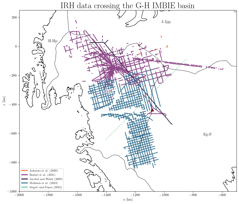
_images/8c993d0200e0a3252f1382d2be4385a2d2604914b6ad3d43c44265a5a7dde8ab.png

Note: all flight lines in the database are associated with one or several IMBIE basin(s). This depends if the flight line crosses one or multiple basins. The plot above shows all the flight lines which have traced IRH data and that crosses at some point the G-H basin.

Plot variables#

Example of plotting the IRH depth of a specific layer found across multiple datasets. Here we still select a range of ages close from each other, which could be attributed to the same layer (but different dating method used maybe). Note the warning in the case, but we can ignore it:

results = db.query(age='37500-38500', var='IRH_DEPTH')
db.plot.var(results, title='AntArchitecture 38ka isochrone depth',
                downsampling_factor=10, # downscale the datasets n times, which makes little visual difference but lighter to plot
                xlim=(-500, 2400),
                ylim=(-2200, 2200),
                scale_factor=0.7, # adjust the size of the plot 
                marker_size=1.2,
                # save='AntA_38ka_depth.png'
                )

WARNING: Multiple layers provided:  ['37600', '38000', '38100', '38200', '38500'] 
Select a unique age for better results

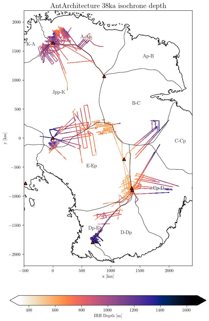
_images/18a8f9fc7087ef9df0a854ac6f05b958914f0af903989dfdde28773d746f7659.png

The above plot shows the absolute IRH depth relative to the ice surface as it is traced. It is often more informative to look at the IRH fraction depth: the depth of a layer relative to the ice thickness (IRH_DEPTH/ICE_THK*100). The fraction depth variable is not directly stored in the database to reduce disk usage. It is probably more efficient to compute it when needed. For this, use the option fraction_depth=True:

# %matplotlib widget
%matplotlib inline
results = db.query(age=['37600', '38000', '38100', '38200', '38500'], var='IRH_DEPTH')
db.plot.var(results, 
            fraction_depth=True,
            title='AntArchitecture 38ka isochrone fractional depth',
                downsampling_factor=10, # downscale the datasets n times, which makes little visual difference but lighter to plot
                xlim=(-500, 2400),
                ylim=(-2200, 2200),
                scale_factor=0.7, # adjust the size of the plot 
                marker_size=1.2,
                # save='AntA_38ka_depth.png'
                )

WARNING: Multiple layers provided:  ['37600', '38000', '38100', '38200', '38500'] 
Select a unique age for better results

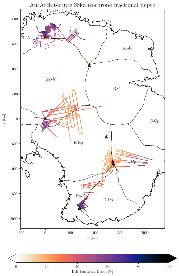
_images/b1f66d63fb992a58c5fce52d9994e742895dea9062feda0bfa2216f614edb944.png

Note that if the variable ICE_THK is not present in a dataset, the fractional depth cannot be computed. In the case, NaN values will be generated instead without warning. So if you get a blank plot, please check if the dataset you queried contains the ICE_THK with db.query(dataset='Author_YYYY').

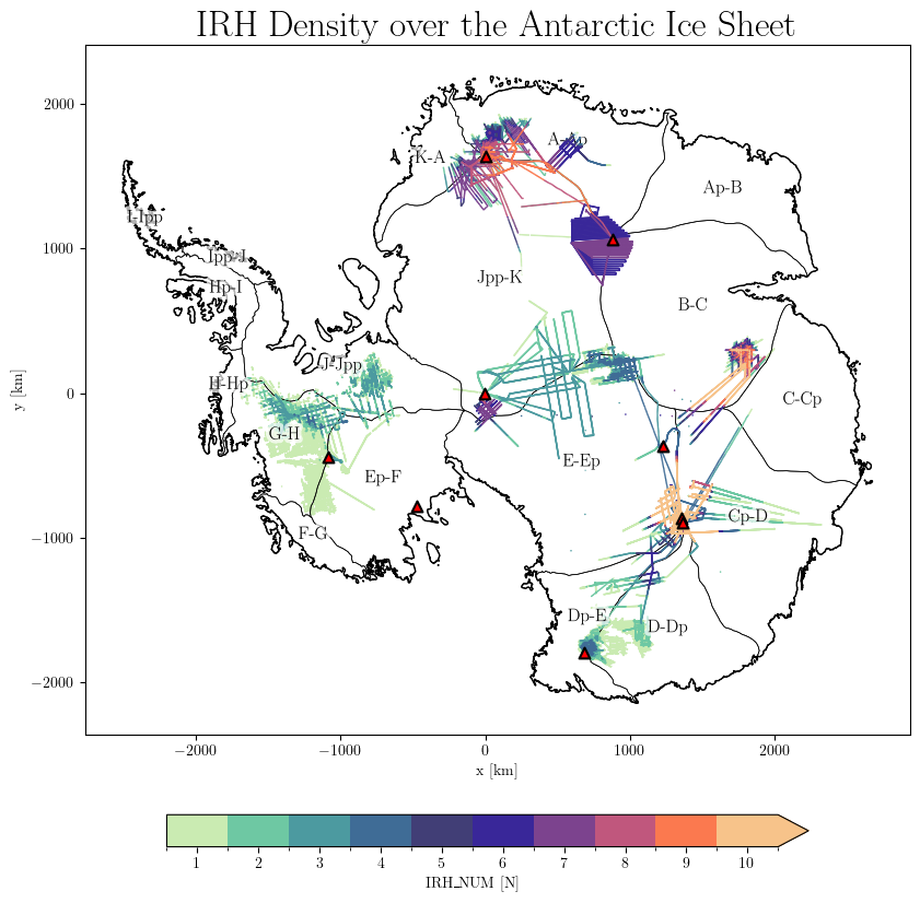
The IRH_NUM variable shows the number of traced isochrones (layers) per data point:

results = db.query(var='IRH_NUM')
db.plot.var(results, title='IRH Density over the Antarctic Ice Sheet',
                downsampling_factor=100,
                scale_factor=1,
                marker_size=1.2,
                )

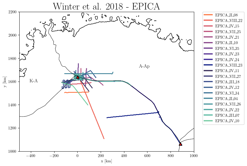
_images/2a87a78f8643f596c882a77ef2eb1c394e78a7e77930d8e579e7201b698ff86f.png

Plot flight IDs#

This plot is useful when we want to identify a specific flight line. One can then identify a flight line of interest on the 2D map, then plot the traced IRHs along the transect (see below):

results = db.query(dataset='Winter%', flight_id=['EPICA%'])
db.plot.flight_id(results, title='Winter et al. 2018 - EPICA',
                xlim=(-500, 1000),
                ylim=(1000, 2200),
                marker_size=1.2,
                )

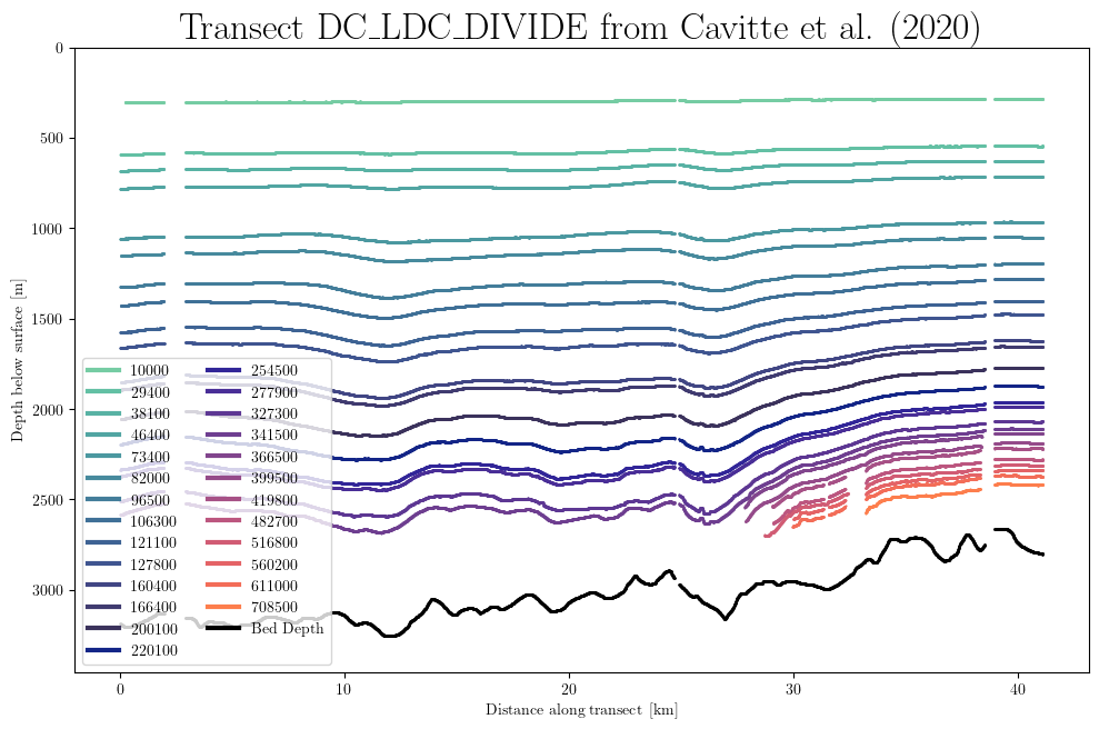
_images/2efb7274d6ee92b883ff8541afb0cde452740cbd460ab472f708d2e9d83783c3.png

Plot layer depths along transect#

results = db.query(dataset='Cavitte_2020', flight_id='DC_LDC_DIVIDE')
db.plot.transect_1D(results)

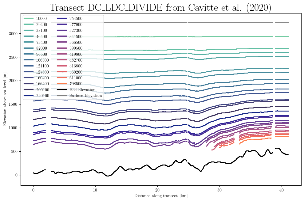
_images/ab26138a8a401b16446a54c30658732d0f20ceb74c0d528f6025ff8630dc8cfb.png

Use the elevation=True option to plot the transect in absolute elevation above sea level:

db.plot.transect_1D(results, elevation=True)

_images/81d9490d69bd98f547c88507048c374b7d1dbba4205db9e4134e102104631e1e.png

Other possible arguments for the plot methods:

cmap: provide your colormap of choice (as LinearSegmentedColormap). Tip: ‘import colormaps as cmaps’ for a large choice of colormaps (see Colormaps docs
vmin and vmax: sets the minimum and maximum values for the colorbar.

BEDMAP#

The AntADatabase now contains all the BEDMAP (1, 2 and 3) data. This is useful to see the whole extent of the existing radar data, or to reconnect the IRH datasets to BEDMAP in order to get the Bed Elevation or Ice Thickness when those are not included.

By default, BEDMAP is not shown in the query, since it is not an IRH dataset. To include it, initialize the Database with the option:

db = Database('/home/anthe/documents/data/isochrones/AntADatabase/', include_BEDMAP=True)

Get files from the database#

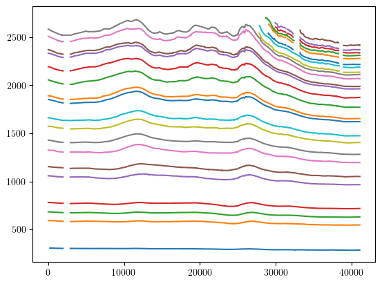
You may want to make your own plots or further process the data after querying the database. One option is to get the list of the files from your query and open them individually with either xarray or h5py. For this, use the get_files() function:

import xarray as xr
import matplotlib.pyplot as plt
results = db.query(dataset='Cavitte_2020', flight_id='DC_LDC_DIVIDE')
file_list = db.get_files(results)
f = file_list[0]
ds = xr.open_dataset(f, engine='h5netcdf')
print(ds)
plt.plot(ds.Distance, ds.IRH_DEPTH)
plt.show()

<xarray.Dataset> Size: 2MB
Dimensions:      (point: 7882, IRH_AGE: 26)
Coordinates:
  * point        (point) int64 63kB 0 1 2 3 4 5 ... 7877 7878 7879 7880 7881
  * IRH_AGE      (IRH_AGE) int64 208B 10000 29400 38100 ... 560200 611000 708500
Data variables:
    PSX          (point) float64 63kB ...
    PSY          (point) float64 63kB ...
    ICE_THK      (point) float64 63kB ...
    BED_ELEV     (point) float64 63kB ...
    SURF_ELEV    (point) float64 63kB ...
    IRH_DEPTH    (point, IRH_AGE) float64 2MB ...
    IRH_AGE_UNC  (IRH_AGE) int64 208B ...
    Distance     (point) float64 63kB ...
    IRH_NUM      (point) int32 32kB ...
Attributes:
    dataset:           Cavitte_2020
    institute:         ['UTIG-AAD', 'NASA-CRESIS', 'BAS']
    project:           ['ICECAP-OIA', 'OIB', 'BE-OI']
    radar instrument:  nan
    acquisition year:  none
    flight ID:         DC_LDC_DIVIDE
    flight ID flag:    original
    DOI dataset:       https://doi.org/10.15784/601411
    DOI publication:   https://doi.org/10.5194/essd-13-4759-2021
    IMBIE_basins:      {"E-Ep": "EAIS", "Cp-D": "EAIS"}

_images/576c51fa84a723df50f7b8e7decb0cd9546708d76e0e37cc69127d356a5e038e.png

xarray provides a nice interface for interacting with the data. This works great when dealing with one file, and for example quickly plot all the layers (see above). But xarray adds some overload, which feels slow when reading many files. h5py on the other hand reads the underlying data right away, which is much more efficient:

import h5py
import matplotlib.pyplot as plt
results = db.query(dataset='Cavitte_2020')
file_list = db.get_files(results)
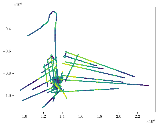
for f in file_list:
    with h5py.File(f, 'r') as ds:
        plt.scatter(ds['PSX'][:], ds['PSY'][:], c=ds['ICE_THK'][:], s=1)
plt.show()

_images/291bfadf55f1dea89a66b022d5770b91b31ff045f27d6cff5a021876b79e2dd4.png

Generate data from the database#

Note: This part could be developed further in the future if there is the need. But for now, I am designing a separate Python module for constraining my ice sheet model of use, which is tailored to this database and other parallel processing libraries. However, the Model-comparison section already give some bits of code about it.

The data_generator() function reads the query and ‘yield’ the dataframes for later use. It uses h5py to read all the data efficiently, and creates pandas dataframes, including all the variables and ages from the query. Columns for IRH DEPTH are named after the age. Basically, it reads the data with h5py as shown above and restructure it as bit, which can be easier to manage layers than with h5py dimensions. Here is a quick example of how this can be used for computing the mean layer depth:

results = db.query(age=['37600', '38000', '38100', '38200', '38500'], var='IRH_DEPTH')
lazy_dfs = db.data_generator(results)

import numpy as np
mean_depth_trs = []
min_depth = float('inf')
max_depth = float('-inf')
for df, md in lazy_dfs:
    depth_values = df[md['age']].values
    mean_depth_trs.append(np.nanmean(depth_values))
    min_depth = min(min_depth, np.nanmin(depth_values))
    max_depth = max(max_depth, np.nanmax(depth_values))


mean_depth = np.nanmean(mean_depth_trs)
std_dev = np.nanstd(mean_depth_trs, ddof=1)
print(f"The mean depth of the 38ka isochrone across East Antarctica is {round(mean_depth, 2)} m ranging from {round(min_depth, 2)} m to {round(max_depth, 2)} m.")

The mean depth of the 38ka isochrone across East Antarctica is 1094.54 m ranging from 210.9 m to 2352.19 m.

Note that the data_generator returns a simple pandas DataFrame for each flight line, containing all queried variables and ages (if exist). The IRH depth of each layer is stored by columns named by age (so the IRH_DEPTH of the layer 38000 is df[‘38000’]). As shown above, one can use the metadata (md) of the current dataframe (df) to get its age (md[‘age’]). Furthermore, if one needs the fraction depth, one can compute it using the ICE_THK (has to be included in the query), or the data_generator has this option: db.data_generator(results, fraction_depth=True). With this option, the layer columns will now be IRH fraction depth instead of absolute IRH_DEPTH.

Pro tips#

The Database methods always keep the last query in memory. This means that one does not have to actually pass argument. Example:

db.query(var='IRH_NUM')
# db.plot.var() # This is equivalent to the overview plot above. Note that without downscaling it is very heavy to plot.

import numpy as np
mean_density_trs = []
min_density = float('inf')
max_density = float('-inf')
for df, md in db.data_generator():    # without explicitly passing results, it uses the last query.
    density_values = df['IRH_NUM']
    mean_density_trs.append(np.mean(density_values))
    min_density = min(min_density, min(density_values))
    max_density = max(max_density, max(density_values))

mean_density = np.mean(mean_density_trs)
print(f"The average number of picked layers per data point in the AntADatabase is {int(mean_density)}, ranging from {int(min_density)} to {int(max_density)}. ")

The average number of picked layers per data point in the AntADatabase is 7, ranging from 1 to 26. 